Introduction to Generalised Additive Models (GAMs)

Linear models are considered multi-purpose since they may be fine-tuned in a variety of ways to adapt to a variety of circumstances and data kinds.

GAMs (Generalized Additive Models) are a type of adaptation that allows us to model non-linear data while keeping it explainable. When compared to Generalised Linear Models like Linear Regression, a GAM is a linear model with a key difference. Non-linear characteristics can be learned by a GAM.

To do this, Linear Regression’s beta coefficients are substituted with a flexible function that allows for non-linear correlations. A spline is the name for this flexible function. Splines are multi-dimensional functions that let us represent non-linear interactions for each feature. A GAM is formed by the sum of multiple splines. The outcome is a highly flexible model that retains some of the linear regression’s explainability.

The requirement that the connection is a simple weighted sum is relaxed in GAMs, which assume that the outcome can be characterized by a sum of arbitrary functions of each variable.

Because we have non-linear distributions, in reality, linear regression is not necessarily a fair depiction of what we perceive. A linear relationship is sometimes a fair, adequate estimate, but it isn’t always. It can’t actually be utilized as a regression model because it doesn’t always reflect the link between the data.

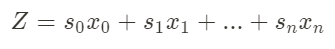
The sum of a linear combination of variables is used to define the Linear Regression equation. Each variable is assigned a weight, and the total is added.

In GAMs, the assumption that our target can be calculated using a linear combination of variables is dropped by simply using a non-linear combination of variables, denoted by s, for ‘smooth function.’

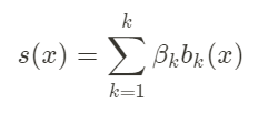
The smooth function is described by the following equation, where β signifies a weight. The other term is b, which stands for basis expansion. A basis expansion is a polynomial expansion that takes the values  x⁰, x¹, x², and so on. 

The great thing about this is that each variable in the equation can have k weights and functions. This method is far more adaptable and less linear than linear regression. A spline is another name for this smooth function. Spline functions can be defined in a variety of ways, which might be confusing. It’s still a popular topic of research to learn more about all the different ways to describe splines. Splines are polynomial functions with a restricted range of values. They can have a variety of appearances, including being linear.

When it comes to estimating non-linear functions, the GAM is far superior. There is no trace of Runge’s Phenomenon as it follows the curve on the expected points. When we utilize high-order polynomials, the edges of the function can oscillate to extreme values, according to Runge’s Phenomenon, which means that models with polynomial features don’t always lead to superior values.

In a GAM model, many splines are used. A weight is assigned to each spline function. To understand what the model is doing over time, we can multiply the function output by the coefficients. The curve is nothing more than the sum of the splines. GAMs are simple to use and can be applied to a variety of variables. You can also choose the number of splines per variable. Variable interactions can also be manually programmed.

The more splines in a model, the wigglier the line becomes in relation to the feature. The problem is that it will begin to overfit the data. The right amount of splines must be discovered so that the model can learn the problem while also being able to generalize successfully. To discover the model that generalizes the best, a typical rule of thumb is to utilize a large number of splines and cross-validate lambda () values. Remember that in a GAM model, you can use different splines and lambda values for each variable.

Link functions, like conventional GLMs, can be used for a variety of distributions, for example, the Logit function for classification problems or Log for a log transformation. Different distributions can be chosen, such as Poisson, Binomial, and Normal.

Here’s how to use PyGAM to fit a GAM. This assumes that the data has been cleaned and preprocessed and is ready to model, with training and test datasets already separated.

import numpy as np
import pandas as pd
from pygam import GAM, LinearGAM, s, f, te
# your training and test datasets should be split as X_train, X_test, y_train, y_test
n_features = 1 # number of features used in the model
lams = np.logspace(-5,5,20) * n_features
splines = 12 # number of splines we will use
# linear GAM for Regression
gam = LinearGAM(
                s(0,n_splines=splines))
     .gridsearch(
                X_train.values, 
                y_train.values,
                lam=lams)
gam.summary()
print(gam.score(X_test,y_test))

PyGAM has a lot more depth because it supports a wide range of GAM types. Take a look at the PyGAM documentation to learn about the many types of GAM (for example, classification) and plot types available.

References: https://towardsdatascience.com/generalised-additive-models-6dfbedf1350a